Due to difficulties encountered with saving and publishing posts here in blogspot, I've decided to use wordpress instead.
Posts are in the process of being transferred to http://cheyabu.wordpress.com.
Thursday, September 23, 2010
Thursday, July 8, 2010
Activity 4 : Area Estimation for Images with Defined Edges
Area estimation plays a crucial role in a number of studies like in the identification of infected cells, estimation of land area and inspection of circuit elements [1]. But of most the time, the subject of these works are either too small (i.e. cells, circuit elements), too large (i.e. land) or too complex (i.e. cells that are not perfect ellipses, land with a rugged border). And physically measuring their dimensions may require too many resources that makes the task nearly impossible.
But but...with the image processing tools that we have now, no object is too small, too big, too many or too complex. An image of our subject and some working knowledge of Green's Theorem is all that we need to have a fairly accurate estimate of an object's area.
Consider a region R whose contour is taken in the counterclockwise direction as shown below. We let F1 and F2 be continuous functions having continuous partial derivatives everywhere in the region R.

Figure 1. Region R
Relating a double integral to a line integral, we get [1]
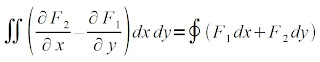
And if we choose F1 = 0, F2 = x, F1 = -y and F2 = 0, the above equation will yield [1]

By averaging the equations above, we get the area A of region R as shown below [1].

If there are Nb pixels in the boundary or contour of region R, then the area A of R is [1]

To first test the implementation of the Green's Theorem, I used the code in Activity 2 to generate basic images with analytically known areas. Since the images I'm using is binarized, another way of computing for the area of my target object is by getting the sum of the pixels in my region R by using the sum(im) function where im is my binarized image. I then compare the accuracies of the areas computed using the Green's Theorem technique and the summing technique with my analytic result. From BA, I got the idea of also exploring the accuracies of these methods as the image dimensions are scaled. These I do for two images, that of a centered circle and a square aperture. The code I've for this part of the activity is shown below.


Assigning new values to a variable does not really clear the variable of its previous contents. When I run the program using a different image but the same variable names, I encounter this error

To address this, I first clear the contents of my variables at the start of my program before using them as shown below.
The circle images I used and the areas I got using the analytic, summing and Green's Theorem methods together with the accuracies of the two computational methods are shown below.
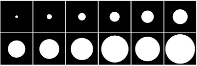
Figure 2. Circle Images with Radius from 0.5 in to 3 in
Table 1. Area of a Circle with Different Radius
The square images I used and their corresponding areas gotten using the process outlined above is as follows.

The summary of the results of the summing and Green's theorem methods for the circle and square images of varying dimensions are shown below.

[2] A. Taylor, "Disaster unfolds slowly in the Gulf of Mexico", The Big Picture, retrieved June 29, 2010 from http://www.boston.com/bigpicture/2010/05/disaster_unfolds_slowly_in_the.html.
[3] "Timeline: Gulf of Mexico oil spill", ABS-CBN news.com, retrieved June 29, 2010 from http://www.abs-cbnnews.com/global-filipino/world/06/01/10/timeline-gulf-mexico-oil-spill.

Table 2. Area of a Square with Different Length

The summary of the results of the summing and Green's theorem methods for the circle and square images of varying dimensions are shown below.

Figure 4. Scaling of Area Estimation
In computing for the area of an object in an image using Green's Theorem, the border or the pixels in the contour are not included in the calculations. Hence, the observed deviation from the analytic area of the target object. This deviation from the theoretical value of the area decreases exponentially as we increase the dimensions of the object as a result of the increase in the surface-to-perimeter ratio. We also see that if the radius of the circle or if half the length of the square is less than 1.00, the computed percent difference for the area of a circle or a square is approximately the same. But as we increase these dimensions, the deviation of the computed area for a square becomes less than that of a circle. We may attribute this to the fact that for a given circle diameter or square length, the perimeter of a circle is greater than a square's perimeter.
When using the sum() function to compute for the area, we get a 100% accuracy for a square. For a circle, on the other hand, we get an almost constant error of 0.20% +/- 0.01%. If we look at the edge of the circle image as shown below, we see that the border is rugged and not smooth. Since every pixel counts in this method, the rugged edge results to the observed error.


Googlemap offers mapping resouces in response to the Gulf of Mexico oil spill crisis. The observed area covered by the oil spill in the gulf is provided by NOAA-NESDIS and can be downloaded from the Google Crisis Response site. An animation of the spread of the oil spill over the gulf for the period May 01 - May 06 is shown below.


There is an observable discrepancy between the areas measured by the summing method and Green's Theorem method. Aside from the earlier stated effect of the exclusion of the border in the Green's Theorem method, there were also some pixels that are not connected to the biggest component and these were also excluded by the follow() function in its tracing of the edge. In cases like this when the areas are too complex, the summing function is more reliable.
Nonetheless, the trends in the spreading of the oil spill in both methods are similar. A decrease in the area covered by the spill is observed on May 4. We can attribute this to the fact that Obama visited the site on May 03 and BP subsequently issued a statement of May 4 stating that cleanup operations were working [3]. Around May 05 - May 06, the weather pattern was reported to be bringing winds of high velocities and as seen above, this may have caused the further spreading of the oil spill [3].
With a little modification of the code, we may further trace the spread of the oil spill to later dates. Knowing how the spill is behaving in response to weather patterns and cleanup operations can help make efforts of saving the gulf more efficient.
Since I gave a thorough explanation of the ways of how we can estimate areas and discussed some of their limitaions, I give myself 10/10.
[1] M. Soriano, "A4-Area Estimation for Images with Defined Edges", AP 186 Handout (June 2010).When using the sum() function to compute for the area, we get a 100% accuracy for a square. For a circle, on the other hand, we get an almost constant error of 0.20% +/- 0.01%. If we look at the edge of the circle image as shown below, we see that the border is rugged and not smooth. Since every pixel counts in this method, the rugged edge results to the observed error.

It is also seen that as the dimensions are increased, not only do the accuracies of the areas computed using the Green's Theorem and the summing method increases but the two methods also approach approximately the same level of accuracy. In general however, the summing method still performs better than the Green's theorem method. Using these methods we have established, we can now compute for areas of more complex shapes with no known analytic solution.
Area estimation can play a crucial role not only in researches performed inside the laboratory but it can also be useful in efforts to hamper potentially harmful effects of an "unprecedented environmental disaster" [2]. Last April 20, a blast on the Deepwater Horizon drilling rig licensed to the BP oil company at the Gulf of Mexico triggered millions of liters of oil to spill over 100 miles of coastline [3].

Figure 6. Gulf of Mexico Oil Spill.
Images taken from http://www.boston.com/bigpicture/2010/05/disaster_unfolds_slowly_in_the.html.

Figure 7. Gulf of Mexico Ecosystem Endangered by the Spill.
Images taken from http://www.boston.com/bigpicture/2010/05/disaster_unfolds_slowly_in_the.html.
The extent of the damage continues to endanger the ecosystem of the Gulf of Mexico [3]. Other oil companies and the US government have joined BP in their attempts to mitigate the spreading of the leak. Containment booms are being erected, protective barriers are being built and devices are being lowered to cap the leaks [2]. To assess the extent to which these efforts are working, tracking the spread and the area covered by the spill is one of the tasks continuously undertaken by experts involved in the control and containment of this disaster [2]. Automating the task of observing the spread of the spill will give the experts more time to actually work on the oil spill cleanup drive. It is here where we can utilize the techniques we've explored earlier concerning area estimation.
Googlemap offers mapping resouces in response to the Gulf of Mexico oil spill crisis. The observed area covered by the oil spill in the gulf is provided by NOAA-NESDIS and can be downloaded from the Google Crisis Response site. An animation of the spread of the oil spill over the gulf for the period May 01 - May 06 is shown below.

Images taken from http://www.google.com/crisisresponse/oilspill/.
The oil spill is shown in green. Using the impixel() function in Matlab, I saved the value of a pixel in the oil spill region in the image. I then scanned the whole image and binarized it such that only areas having pixel values equal to that I saved will be shown in white. The result of this binarization is shown below.

Using the follow() function in Scilab, I then traced the contour for the coordinates of the border. This is necessary for the application of the Green's Theorem method in the estimation of the area.

Figure 10. Edge of Observed Oil Spill in the Gulf of Mexico. (Click to view animation)
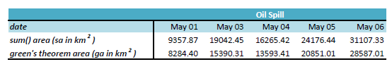
I used the two methods developed earlier, the summing method and the Green's Theorem method for the estimation of the area covered by the oil spill. The results of which are shown below.
Table 3. Observed Oil Spill in the Gulf of Mexico

Figure 11. Observed Oil Spill in the Gulf of Mexico
There is an observable discrepancy between the areas measured by the summing method and Green's Theorem method. Aside from the earlier stated effect of the exclusion of the border in the Green's Theorem method, there were also some pixels that are not connected to the biggest component and these were also excluded by the follow() function in its tracing of the edge. In cases like this when the areas are too complex, the summing function is more reliable.
Nonetheless, the trends in the spreading of the oil spill in both methods are similar. A decrease in the area covered by the spill is observed on May 4. We can attribute this to the fact that Obama visited the site on May 03 and BP subsequently issued a statement of May 4 stating that cleanup operations were working [3]. Around May 05 - May 06, the weather pattern was reported to be bringing winds of high velocities and as seen above, this may have caused the further spreading of the oil spill [3].
With a little modification of the code, we may further trace the spread of the oil spill to later dates. Knowing how the spill is behaving in response to weather patterns and cleanup operations can help make efforts of saving the gulf more efficient.
Since I gave a thorough explanation of the ways of how we can estimate areas and discussed some of their limitaions, I give myself 10/10.
[2] A. Taylor, "Disaster unfolds slowly in the Gulf of Mexico", The Big Picture, retrieved June 29, 2010 from http://www.boston.com/bigpicture/2010/05/disaster_unfolds_slowly_in_the.html.
[3] "Timeline: Gulf of Mexico oil spill", ABS-CBN news.com, retrieved June 29, 2010 from http://www.abs-cbnnews.com/global-filipino/world/06/01/10/timeline-gulf-mexico-oil-spill.
Saturday, June 26, 2010
Activity 3 : Image Types and Formats
Images are not only our way of remembering scenes we've seen but through the pictures we've captured, we can let others also live the moments we've experienced. Understanding the different types and formats of images may seem like a stuff for the geeks. But the knowledge of the different ways of presenting and storing images will help in building the story we want to tell. Yes, "geekiness" can make things more interesting! :D
So here's the start of my attempt to be a poetic imaging geek...
There are four basic types of images, namely Binary, Grayscale, Truecolor and Indexed images. Each type differ in size and in the range of values their pixels can have. The description for each of these types and examples of them are given below.
Binary Images
Binary image file size:
an image of size 256x256 pixels == an image file size of 256x256 bits or 8Kb
A Binary Image as its name suggests is binarized, it contains only two values. They present scenes in black and white or 1's and 0's. Some may ask, how about the values in between? Why reduce things to just ones and zeros? But then... sometimes more is seen with less.
In some cases, we are after the lines and shapes contained in an image. In this instances, having binarized values helps reveal these lines and shapes that are otherwise concealed by the other more "enthralling" aspects of the image. Some works that benefits from having binary images are those involving the identification of roofs or particle tracks and those making use of fingerprints, line art and signatures.
Below is an example of a binary image and the result of an imfinfo() query in Scilab. As can be seen below, there are only two colors in the image.
Figure 1. Binary Image.
Size: 362 rows X 362 columns
Indexed Image
FileName: bw.gif
FileSize: 4219
Format: GIF
Width: 362
Height: 362
Depth: 8
StorageType: indexed
NumberOfColors: 2
ResolutionUnit: centimeter
XResolution: 72.000000
YResolution: 72.000000
Grayscale Images
Grayscale image file size:
an image of size 256x256 pixels == an image file size of 65,536 bytes or 64Kb
A Grayscale image contains pixel values anywhere in the range [0,256]. Unlike in binary images, in grayscale, a gradient of color tones is now available. Distinctions, boundaries and lines are not always sharp but may now be blurred. But unlike in binary images, differences in density is more apparent in grayscale images. More details about the composition of items in the image can be investigated. This is particularly essential in medical or biological imaging and face recognition.
Below is an example of a grayscale image and the result of an imfinfo() query in Scilab. As expected, we see from the query that the number of colors of the image below is 256.

Figure 2. Grayscale Image.
Size: 600 rows X 800 columns
Indexed Image
FileName: x8HePD2z96890635_800x600.jpg
FileSize: 113873
Format: JPEG
Width: 800
Height: 600
Depth: 8
StorageType: indexed
NumberOfColors: 256
ResolutionUnit: inch
XResolution: 72.000000
YResolution: 72.000000
Truecolor Images
Truecolor image file size:
an image of size 256x256 pixels == an image file size of 256x256x3 = 196608 bytes or 192Kb
Truecolor images add dimensions to images. Here, pixels are not just black and white or gradients of tones but are products of three channels combined. Each pixel has a corresponding red, green and blue values with each channel falling in the range [0,256]. This is the type of image, we are most familiar with as its appearance resembles the actual scenes we took and its method of color storage is intuitive (our coloring lessons as a child have taught us that another color can be produced by combining two or more colors). Images taken by digital cameras are usually by default of this type.
Below is an example of a truecolor image and the result of an imfinfo() query in Scilab. The number of colors that the query gave for the image below was zero. Since this intrigued me, I tried other truecolor images and the number of colors was still zero. I found out from http://siptoolbox.sourceforge.net/doc /sip-0.2.0-reference/imfinfo.html, that the NumberOfColors of a truecolor image is always given as zero.

Figure 3. Truecolor Image.
(Image taken from one of albums during a summer vacation in Pangasinan)
Size: 3 X 1728 rows X 2304 columns
Truecolor Image
FileName: CIMG1961.JPG
FileSize: 1593714
Format: JPEG
Width: 2304
Height: 1728
Depth: 8
StorageType: truecolor
NumberOfColors: 0
ResolutionUnit: inch
XResolution: 72.000000
YResolution: 72.000000
Other examples of Truecolor Images (I found a lot of old pictures I like while looking for a sample image to use):
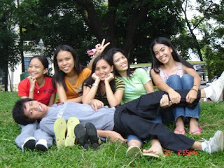


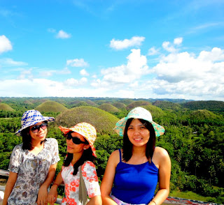
Figure 4. Samples of Truecolor Images.
Indexed Images
Indexed Images are like Truecolor Images in that they are similar in appearance. But in Indexed images, colors are represented as numbers denoting an index in a colormap, much like a directory. An image is sometimes chosen to be stored indexed since they are generally smaller in size as compared to truecolor images.
Below is an example of an indexed image and the result of an imfinfo() query in Scilab. The number of colors that the query gave for the image below was 256 since each channel can take one of 256 values.

Figure 5. Indexed Image.
(Image taken from http://www.eso.org/sci/data-processing/software/scisoft/rpm2html/fc6/scisoft-idl-7.0.0-0i386.html)
Size: 248 rows X 248 columns
Indexed Image
FileName: imgcolor16.gif
FileSize: 27065
Format: GIF
Width: 248
Height: 248
Depth: 8
StorageType: indexed
NumberOfColors: 256
ResolutionUnit: centimeter
XResolution: 72.000000
YResolution: 72.000000
With the improvement of imaging techniques and with the advent of new problems that need to be solved, advanced image types were also developed as listed below.
High Dynamic Range (HDR) Images
According to http://brajeshwar.com/2006/what-are-hdr-or-high-dynamic-range-images/, HDR images "can store pixel values that span the whole tonal range of the real-world which are quite high,in the range of 100,000:1". 32-bit images are usually considered as HDR. Each pixel value in an HDR image is proportional to the amount of light in the scene as captured by the camera.
Below is an example of an HDR image. The details in the image is more defined and the colors are brighter as compared to Truecolor Images which are in the Low Dynamic Range.
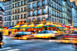
Figure 6. High Dynamic Range Image.
Multi or Hyperspectral Images
These kind of images have bands that are more than three. Since they have higher spectral resolution, they are important for works which involves spectral characterization such as the identification of material properties. The number of channels of a multispectral image is in the order of 10's while that of a hyperspectral image is in the order of 100.
Below is an example of a hyperspectral image. As can be seen, the surfaces in the image below is well-defined.
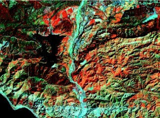
Figure 7. Hyperspectral Image.
3D Images
The 3D information of a scene can be captured and stored by having point clouds defining (x,y,z), stacking 2D images of several cross-sections or by taking stereopairs which are dual images of a scene taken a short distance apart.
Below is an example of a 3D image which utilizes the fact that our eyes bend cyan and magenta colors at different angles.

Figure 8. 3D Image.
Temporal Images or Videos
Videos are produced by taking a large number of frames for every millisecond. The high rate at which images are captured produces a seamless stitch of snapshots that make up a video.
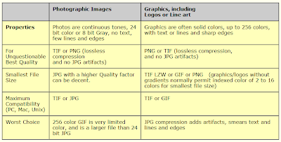
Aside from the image types, the amount of information that is stored in an image also depends on the file format with which it was stored. Below is a table from